Quick Sort

Quick Sort is a sorting algorithm that follows the divide-and-conquer approach to efficiently sort an array or a list of elements. It is based on the principle of partitioning the array into smaller subarrays, sorting them independently, and then combining the sorted subarrays to obtain the final sorted result.

The algorithm works by selecting a pivot element from the array and partitioning the other elements into two subarrays based on their relation to the pivot. Elements less than the pivot are placed in the left subarray, and elements greater than the pivot are placed in the right subarray. The pivot is then in its final sorted position.

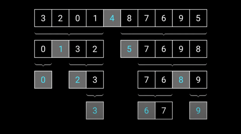
The partitioning step is performed recursively on the subarrays until the base case is reached, which occurs when the subarray contains only one element or is empty. At this point, the subarrays are considered sorted, and they are combined to obtain the sorted array.

The choice of the pivot element is crucial for the efficiency of the Quick Sort algorithm. Ideally, the pivot should be selected in a way that divides the array into two roughly equal-sized subarrays. This helps achieve a balanced partition and ensures a good average-case performance. Various techniques can be used to select the pivot, such as choosing the first, last, or middle element, or using a random selection.

The time complexity of Quick Sort is O(n log n) on average, making it one of the fastest sorting algorithms. However, in the worst case, where the pivot is consistently chosen poorly and the array is already sorted or nearly sorted, the time complexity can degrade to O(n^2). This occurs when the partitioning is highly imbalanced, resulting in one subarray significantly larger than the other.

Quick Sort is an in-place sorting algorithm, meaning it requires only a small amount of additional memory for the recursive calls and pivot selection. This makes it efficient in terms of space complexity, with an average case of O(log n) and a worst case of O(n).

Quick Sort is widely used in practice due to its overall efficiency, simplicity, and good average-case performance. It is suitable for both small and large datasets and is a common choice for sorting applications.

Algorithm

The Quick Sort algorithm can be described using the following steps:

1. Choose a pivot element from the array. The pivot can be selected in different ways, such as choosing the first, last, middle element, or using a random selection.
2. Partition the array by rearranging its elements in such a way that all elements less than the pivot are placed before it, and all elements greater than the pivot are placed after it. The pivot will be in its final sorted position. This step is also known as the partitioning step.
3. Recursively apply the above two steps to the subarray of elements before the pivot and the subarray of elements after the pivot. This effectively divides the array into smaller subarrays.
4. Continue the recursion until the base case is reached, which occurs when a subarray contains only one element or is empty. At this point, the subarrays are considered sorted.
5. Combine the sorted subarrays to obtain the final sorted array.

Here is a Python code example that implements the Quick Sort algorithm:

def quick_sort(arr):
if len(arr) <= 1:
return arr

pivot = arr[0]
left = [x for x in arr[1:] if x <= pivot]
right = [x for x in arr[1:] if x > pivot]

return quick_sort(left) + [pivot] + quick_sort(right)

Example usage

arr = [5, 2, 9, 1, 3, 6]
sorted_arr = quick_sort(arr)
print(sorted_arr)

In this example, the quick_sort function takes an array arr as input and performs the Quick Sort algorithm recursively. The base case is when the length of the array is less than or equal to 1, in which case the array is returned as is.

The pivot is chosen as the first element of the array (arr[0]). The left list is created by collecting all elements less than or equal to the pivot, and the right list is created by collecting all elements greater than the pivot.

The function then recursively calls quick_sort on the left and right subarrays, and combines the sorted subarrays by concatenating quick_sort(left), the pivot, and quick_sort(right).

Finally, the example demonstrates the usage of the quick_sort function by sorting an array [5, 2, 9, 1, 3, 6] and printing the sorted array [1, 2, 3, 5, 6, 9].

Application

The Quick Sort algorithm has several applications and is widely used in various scenarios. Some of the common applications of Quick Sort include:

1. Sorting: Quick Sort is primarily used for sorting arrays or lists of elements. It is known for its efficiency and is often preferred over other sorting algorithms like Bubble Sort or Insertion Sort, especially for large datasets.
2. Programming Languages: Quick Sort is a fundamental algorithm used in programming languages and libraries for their built-in sorting functions. Many programming languages, including Python, C++, Java, and JavaScript, implement Quick Sort as their default sorting algorithm.
3. Database Systems: Quick Sort is utilized in database systems for sorting large amounts of data efficiently. It helps in improving the performance of operations like sorting indexes or performing queries that involve sorting.
4. Computer Science Education: Quick Sort is a classic algorithm and is commonly taught in computer science courses as an introduction to sorting algorithms. It helps students understand the concept of divide and conquer and serves as a foundation for learning more complex algorithms.
5. Numerical Analysis: Quick Sort is used in numerical analysis and mathematical computations for sorting arrays of numbers. It is efficient and well-suited for sorting numerical data sets.
6. File Systems: Quick Sort can be applied to file systems for organizing files based on their attributes like names, sizes, or modification dates. It allows for faster access and retrieval of files by maintaining a sorted order.
7. Data Compression: Quick Sort is utilized in various data compression algorithms, such as Huffman coding, where sorting plays a crucial role in determining the frequency or probability of symbols in a dataset.
8. Network Routing: Quick Sort can be employed in network routing algorithms for determining the shortest or fastest path between network nodes. Sorting helps in organizing routing tables or determining the optimal routing path.

Overall, Quick Sort’s versatility, efficiency, and widespread implementation make it a valuable algorithm in various fields ranging from software development to data analysis and system optimization.

Complexity

The time and space complexity of the Quick Sort algorithm can be summarized as follows:

Time Complexity:

• Best Case: O(n log n)
• Average Case: O(n log n)
• Worst Case: O(n^2)

The time complexity of Quick Sort largely depends on the choice of the pivot element and the input array’s initial order. In the best and average cases, when the pivot selection is optimal and the input array is divided evenly, Quick Sort exhibits a time complexity of O(n log n). This makes it one of the fastest sorting algorithms available.

However, in the worst case scenario, where the pivot is consistently chosen as the smallest or largest element and the input array is already sorted or nearly sorted, Quick Sort can exhibit a time complexity of O(n^2). This worst case occurs when the partition step consistently creates unbalanced partitions, resulting in a large number of recursive calls.

Despite the worst case time complexity, Quick Sort is still widely used due to its average case performance, which is highly efficient for most inputs.

Space Complexity: The space complexity of Quick Sort is generally O(log n) for the recursive calls. It uses the call stack to keep track of the recursive function calls and the corresponding sub-arrays. In the worst case scenario, the space complexity can be O(n) if the partitioning consistently creates unbalanced partitions, leading to a large number of recursive calls.

It’s important to note that Quick Sort is an in-place sorting algorithm, meaning it does not require additional memory proportional to the input size. It rearranges the elements within the given array itself, which makes it memory-efficient.

Overall, Quick Sort’s average case time complexity of O(n log n), combined with its in-place sorting and general efficiency, makes it a popular choice for sorting large datasets. However, its worst case time complexity of O(n^2) should be considered when dealing with input arrays that may already be sorted or nearly sorted.

Coding Example in Python:

def quick_sort(arr):
if len(arr) <= 1: return arr else: pivot = arr[0] lesser = [x for x in arr[1:] if x <= pivot] greater = [x for x in arr[1:] if x > pivot]
return quick_sort(lesser) + [pivot] + quick_sort(greater)

Example usage

arr = [5, 2, 9, 1, 6, 3]
sorted_arr = quick_sort(arr)
print(sorted_arr)

In the above code, the quick_sort function takes an array arr as input and recursively sorts it using the Quick Sort algorithm.

The base case checks if the length of the array is less than or equal to 1, in which case the array is already sorted and can be returned as is.

Otherwise, it selects the first element of the array as the pivot and creates two sub-arrays: lesser containing elements less than or equal to the pivot, and greater containing elements greater than the pivot.

The function then recursively calls quick_sort on the lesser and greater sub-arrays, and concatenates the sorted lesser array, pivot, and sorted greater array to form the final sorted array.

Finally, we demonstrate the usage of the quick_sort function by sorting an example array [5, 2, 9, 1, 6, 3] and printing the sorted result.

Please note that this is a simplified implementation for illustrative purposes. In a production environment, you may want to consider optimizations, such as choosing a better pivot selection strategy (e.g., median-of-three), or handling edge cases for large or duplicate elements.

About The Author